Abstract

The prior distribution is the part of a Bayesian model that most often invites suspicion: “you can make a Bayesian analysis say whatever you want by twisting the prior.” That accusation is sharper than the textbook reply (“priors matter less than you fear, look at the posterior”) suggests, and it is sharper than the casual recipe (“just use a flat prior”) deserves. There are at least five inequivalent answers to “what does an uninformative prior even mean?”, the Jeffreys rule has a beautiful geometric derivation that is rarely spelled out, and improper priors can be perfectly safe or silently wrong depending on the dataset.

We will work through, in order, (i) the conjugate prior framework as an exponential-family construction, (ii) improper priors and the propriety theorem that decides when they are safe, (iii) the taxonomy of uninformative priors and why Laplace’s flat prior is not coordinate-free, (iv) the Jeffreys prior in full multivariate form, with the reparametrization-invariance proof and the KL-maximisation argument, (v) the information geometry picture that makes Jeffreys feel inevitable, (vi) Bernardo’s reference priors and where they disagree with Jeffreys in higher dimensions, (vii) numerical experiments that empirically verify the Bernardo theorem, the frequentist coverage gap between Jeffreys and reference for the Normal model, and the arc-length picture of Jeffreys on the Bernoulli line, and (viii) a worked example on a 10-throw dice problem that re-derives every claim on numbers small enough to check by hand.

Content

code below was written for personal study. There may be mistakes — please leave a comment.

Preliminaries

Bayes’ rule and the role of the prior

Given a sampling model $p(x \mid \theta)$ and a prior $\pi(\theta)$ on the parameter space $\Theta$, Bayes’ rule produces the posterior

$$ p(\theta \mid x) \;=\; \frac{p(x \mid \theta)\,\pi(\theta)}{m(x)}, \qquad m(x) \;=\; \int_\Theta p(x \mid \theta)\,\pi(\theta)\,d\theta. \tag{1} $$

The marginal $m(x)$ — also called the evidence or prior predictive — is the normaliser that makes $p(\theta \mid x)$ a probability density in $\theta$. It is also what makes the choice of prior consequential: if $m(x)$ is finite, the posterior exists and is unique; if not, the posterior is meaningless even though the right-hand side of (1) is well-defined pointwise.

The prior plays two very different roles. The first is the informative role: it encodes whatever the modeller actually knows about $\theta$ before seeing $x$. The second is the regularising role: even when the modeller knows nothing, a prior is still needed to make the right-hand side of (1) a density. Most of the difficulty in this post stems from the gap between these two roles. There is no universally correct prior in the regularising mode, but there are several principled constructions that we can compare on their own terms.

Exponential families and natural parameters

Almost every prior we will meet can be written cleanly in the language of exponential families, so we state the definition up front and reuse it in §3 (conjugate priors), §6 (Jeffreys), and §9 (maximum entropy).

A statistical model $\{p(x \mid \eta)\}$ is an exponential family in natural parametrisation if

$$ p(x \mid \eta) \;=\; h(x)\,\exp\!\bigl\{\eta^{\top} T(x) \;-\; A(\eta)\bigr\}, \qquad A(\eta) \;=\; \log\!\int h(x)\,e^{\eta^{\top} T(x)}\,dx, \tag{2} $$

where $\eta \in \mathbb R^d$ is the natural parameter, $T(x) \in \mathbb R^d$ is the sufficient statistic, $h(x)$ is the base measure, and $A$ is the log-partition function. The cumulant identities

$$ \nabla A(\eta) \;=\; \mathbb E_\eta[T(X)], \qquad \nabla^2 A(\eta) \;=\; \mathrm{Cov}_\eta(T(X)) \tag{3} $$

are derived by differentiating $\int h(x)\,e^{\eta^\top T(x)-A(\eta)}dx = 1$ once and twice in $\eta$. The second identity is the key one for §6: for an exponential family in natural parametrisation, the Fisher information equals the Hessian of $A$, $I(\eta) = \nabla^2 A(\eta)$. This means the Jeffreys prior $\sqrt{\det I(\eta)}$ is computable directly from the log-partition function, without ever evaluating an expectation.

Notation

Throughout, $\theta \in \Theta \subseteq \mathbb R^d$ is the unknown parameter, $x = (x_1, \ldots, x_n) = x^n$ is the observed sample, and $\pi(\theta)$ is a prior density on $\Theta$ (proper or improper). For Beta priors we use the parametrisation $\mathrm{Beta}(\alpha, \beta) \propto \theta^{\alpha-1}(1-\theta)^{\beta-1}$. For Normal data we keep $(\mu, \sigma^2)$ as the parametrisation, switching to $\sigma$ only when explicitly noted. Fisher information matrices use $I(\theta)$; differential entropy uses $h(\pi) = -\int \pi \log \pi$. We cite references by number, e.g. [ref 3], where the bibliography sits at the end of the post.

Conjugate priors

Definition

A family $\mathcal F$ of priors is conjugate to a likelihood family $\mathcal L$ if, for every $\pi \in \mathcal F$ and every likelihood $p(\cdot \mid \theta) \in \mathcal L$, the posterior $p(\theta \mid x) \propto p(x \mid \theta)\,\pi(\theta)$ stays in $\mathcal F$. This is a closure property, not a normative claim: conjugacy says nothing about whether the prior is reasonable, only that it makes the posterior the same shape as the prior.

The exponential-family construction

Conjugacy is not a coincidence. Given an exponential-family likelihood in the form (2), the canonical conjugate prior on the natural parameter $\eta$ is

$$ \pi(\eta \mid \tau_0, \nu_0) \;\propto\; \exp\!\bigl\{\tau_0^{\top} \eta \;-\; \nu_0\, A(\eta)\bigr\}, \tag{4} $$

where $\tau_0 \in \mathbb R^d$ and $\nu_0 > 0$ are hyperparameters. To see why (4) is conjugate, take a sample $x_1, \ldots, x_n$, sum the sufficient statistics to get $S_n := \sum_i T(x_i)$, and multiply the prior by the likelihood:

$$ \begin{aligned} \pi(\eta \mid x^n) &\;\propto\; \pi(\eta \mid \tau_0, \nu_0) \prod_{i=1}^n p(x_i \mid \eta) \\ &\;\propto\; \exp\!\bigl\{\tau_0^{\top}\eta - \nu_0\,A(\eta)\bigr\} \cdot \exp\!\bigl\{S_n^{\top} \eta - n A(\eta)\bigr\} \\ &\;=\; \exp\!\bigl\{(\tau_0 + S_n)^{\top}\eta \;-\; (\nu_0 + n)\,A(\eta)\bigr\}. \end{aligned} \tag{5} $$

So the posterior has the same shape (4) with updated hyperparameters

$$ \tau_n \;=\; \tau_0 + S_n, \qquad \nu_n \;=\; \nu_0 + n. \tag{6} $$

This is the entire conjugate prior recipe. The hyperparameter pair $(\tau_0, \nu_0)$ has a sufficient-statistic interpretation: $\tau_0$ acts like a pseudo-count of the sum of statistics, and $\nu_0$ acts like a pseudo-sample-size. As $n \to \infty$, the data hyperparameters $(S_n, n)$ dominate and the prior’s influence vanishes at rate $\nu_0 / (\nu_0 + n) = O(n^{-1})$.

Five worked examples

Likelihood	Sufficient stat $T$	Natural conjugate prior on parameter	Posterior update
$\mathrm{Bernoulli}(\theta)$	$T(x) = x$	$\mathrm{Beta}(\alpha, \beta)$ on $\theta$	$\alpha\!\to\!\alpha + \sum x_i$, $\beta\!\to\!\beta + n - \sum x_i$
$\mathrm{Poisson}(\lambda)$	$T(x) = x$	$\mathrm{Gamma}(\alpha, \beta)$ on $\lambda$	$\alpha\!\to\!\alpha + \sum x_i$, $\beta\!\to\!\beta + n$
$\mathcal N(\mu, \sigma^2)$, $\sigma^2$ known	$T(x) = x$	$\mathcal N(\mu_0, \tau_0^2)$ on $\mu$	precision-weighted update
$\mathcal N(\mu, \sigma^2)$, $\mu$ known	$T(x) = (x-\mu)^2$	$\mathrm{Inv\text{-}Gamma}(\alpha, \beta)$ on $\sigma^2$	$\alpha\!\to\!\alpha + n/2$, $\beta\!\to\!\beta + \tfrac12 \sum (x_i-\mu)^2$
$\mathrm{Multinomial}(K, p)$	$T(x) = (\mathbf 1_{x=k})_{k=1}^{K}$	$\mathrm{Dirichlet}(\alpha_1, \ldots, \alpha_K)$ on $p$	$\alpha_k\!\to\!\alpha_k + n_k$

Walking through the Beta–Binomial row: with $\mathrm{Beta}(\alpha, \beta)$ prior and Binomial$(n, k)$ data the posterior is $\mathrm{Beta}(\alpha + k,\,\beta + n - k)$. The posterior mean

$$ \mathbb E[\theta \mid x] \;=\; \frac{\alpha + k}{\alpha + \beta + n} \;=\; \frac{\alpha + \beta}{\alpha + \beta + n}\cdot\frac{\alpha}{\alpha+\beta} \;+\; \frac{n}{\alpha+\beta+n}\cdot\frac{k}{n} \tag{7} $$

is a convex combination of the prior mean $\alpha/(\alpha+\beta)$ and the MLE $k/n$, with weight $\alpha+\beta$ on the prior. This is the shrinkage picture and the cleanest sense in which $\alpha-1, \beta-1$ act as prior pseudo-counts of successes and failures. We visualise this directly in §10 (E5).

When conjugacy is enough, and when it is not

In 2026 the MCMC stack (Stan, PyMC, NumPyro, JAGS, INLA) has eliminated the historical reason for using conjugate priors — that they made the posterior tractable in closed form. The remaining reason to care about conjugacy is pedagogical and theoretical: conjugate priors expose the sufficient-statistic interpretation of the posterior update, give clean limits as $\nu_0 \to 0$ (towards “uninformative” choices), and produce closed-form predictive densities. For genuinely informative priors that do not happen to be conjugate — for example, an industry-domain belief encoded as a mixture of Gaussians — MCMC is the right hammer.

A full table of conjugate pairs across the standard distributions is John D. Cook’s Compendium [ref 3], which we recommend as a desk reference.

Improper priors

Definition

A prior $\pi$ is improper on $\Theta$ if $\int_\Theta \pi(\theta)\,d\theta = \infty$. Three canonical examples:

• The flat prior on the real line: $\pi(\mu) = 1$ for $\mu \in \mathbb R$.
• The scale-invariant prior on the positive line: $\pi(\sigma) \propto 1/\sigma$ for $\sigma > 0$.
• Haldane’s prior on the unit interval: $\mathrm{Beta}(0, 0) \propto \theta^{-1}(1-\theta)^{-1}$ for $\theta \in (0, 1)$.

These do not define probability distributions. The question is whether they nevertheless define legitimate Bayesian updates.

The propriety theorem

The Bayes step (1) divides $p(x \mid \theta)\,\pi(\theta)$ by $m(x) = \int p(x \mid \theta)\,\pi(\theta)\,d\theta$. When $\pi$ is improper, $m(x)$ can still be finite for some observations and infinite for others. The fundamental theorem is:

Propriety. Let $\pi$ be a (possibly improper) prior on $\Theta$ and let $p(x \mid \theta)$ be a sampling model. The posterior $p(\theta \mid x) = p(x \mid \theta)\,\pi(\theta) / m(x)$ is a proper probability density on $\Theta$ if and only if $m(x) < \infty$ for the observed $x$.

Propriety is a property of the combination of prior and observed data, not of the prior alone. This is the textbook gotcha [ref 2, ref 4, ref 6]: improper priors are not in themselves illegitimate, but they require the modeller to check $m(x) < \infty$ on the specific data, every time.

Two worked examples

Bernoulli with Haldane. Take $\pi(\theta) = \mathrm{Beta}(0,0) \propto 1/[\theta(1-\theta)]$ on $(0,1)$. After observing $k$ successes in $n$ Bernoulli trials, the posterior is $\mathrm{Beta}(k, n-k)$, which is proper if and only if $k \ge 1$ and $n - k \ge 1$. If $k = 0$, the unnormalised posterior $\theta^{-1}(1-\theta)^{n-1}$ has $\int_0^1 \theta^{-1}(1-\theta)^{n-1}\,d\theta = \infty$, so the posterior is improper. This failure mode is plotted as Figure e1_haldane_failure.png in §10: the “posterior” mass piles up at $\theta = 0$ and refuses to normalise.

Normal with the Jeffreys joint $1/\sigma^2$. Take $\pi(\mu, \sigma) \propto 1/\sigma^2$ on $\mathbb R \times (0, \infty)$. After observing $n \ge 2$ data points $x_1, \ldots, x_n$ with sample mean $\bar x$ and sum of squares $SS = \sum (x_i - \bar x)^2$, the joint posterior is proper whenever $SS > 0$, which holds with probability one under any continuous sampling model. So in practice Jeffreys joint is fine for $n \ge 2$, but degenerate at $n = 1$.

Lindley–Bartlett: improper priors break model comparison

Improper priors are not fine for one specific purpose: Bayesian model comparison via Bayes factors. The Bayes factor $\mathrm{BF}_{12} = m_1(x)/m_2(x)$ between two models with improper priors has arbitrary numerical value, because $m(x)$ is only defined up to a multiplicative constant (the unspecified normalisation of $\pi$). This is the Lindley–Bartlett paradox [ref 4]: the same data can support model 1 over model 2 by any factor you choose, depending on which improper prior representative you wrote down. The practical implication is that improper priors should never be used for hypothesis testing or model selection, only for parameter estimation within a single model.

When improper is fine

Improper priors are routinely the right answer when (i) the parameter space has a transitive group action (translation on $\mathbb R$, scale on $(0,\infty)$) and we want the prior to respect that symmetry — the right Haar measure of the group is the natural choice, and it is typically improper; (ii) the data carries enough information that $m(x) < \infty$ trivially; and (iii) we are doing parameter estimation, not model comparison. The reference priors of §8 are almost always improper on unbounded parameter spaces, and this is by design.

The noninformative landscape

Laplace’s principle of insufficient reason and why it fails

The oldest proposal for an uninformative prior is Laplace’s principle of insufficient reason: if you have no reason to prefer any value of $\theta$ over any other, take $\pi(\theta) \propto 1$. The principle is intuitive and produces a unique answer once the parametrisation is chosen.

That qualifier — once the parametrisation is chosen — is the problem. Take a one-parameter model with parameter $\theta \in (0, \infty)$ and consider the reparametrisation $\eta = \log\theta \in \mathbb R$. Laplace’s principle applied to $\theta$ gives $\pi(\theta) = c$, which pushes forward to $\pi(\eta) = c \cdot |d\theta/d\eta| = c\, e^{\eta}$ on $\mathbb R$ — not flat. So the flat prior depends on the choice of coordinate: a modeller who parametrises in $\theta$ and a modeller who parametrises in $\eta$, both invoking the same principle of indifference, get incompatible answers.

This single observation is the reason the field needed something better than Laplace, and is what motivates every construction in this post from §6 onwards. We want priors whose definition is intrinsic to the model, not to the parametrisation chosen to describe it.

Five inequivalent answers to “uninformative”

The literature offers at least five inequivalent constructions of “uninformative” priors, each with its own justification:

1. Jeffreys: $\pi_J(\theta) \propto \sqrt{\det I(\theta)}$, where $I$ is the Fisher information matrix. Coordinate-free by construction.
2. Reference (Bernardo): the prior that maximises the asymptotic missing-information functional. Coincides with Jeffreys in one parameter, may differ in higher dimensions.
3. Maximum entropy: maximise $h(\pi) = -\int \pi \log \pi$ (or relative entropy with respect to some base measure) subject to constraints (moments, support).
4. Probability matching: priors whose Bayesian credible intervals have frequentist coverage to high order in $n$.
5. Formal rules (the Berger–Bernardo–Sun family): a small zoo of group-theoretic constructions including right and left Haar measures, MDL priors, and the Yang–Berger catalog [ref 1].

A short comparison on three orthogonal axes:

Construction	Coordinate-free?	Data-dependent?	Unique?
Laplace flat	No	No	Yes (given parametrisation)
Jeffreys	Yes	Yes (via Fisher info)	Yes
Reference (Bernardo)	Yes	Yes	Up to ordering of parameters
Maximum entropy	Yes (with base measure)	No	Yes (given constraints)
Probability matching	Yes	Yes	Often unique only to leading order

We unpack the entries of this table in §6–§9.

Jeffreys prior

Fisher information

For a model $p(x \mid \theta)$ on $\Theta \subseteq \mathbb R^d$ with twice-differentiable log-likelihood, the Fisher information matrix is

$$ I(\theta)_{ij} \;=\; \mathbb E_\theta\!\bigl[\partial_i \log p(X\mid\theta)\,\partial_j \log p(X\mid\theta)\bigr] \;=\; -\,\mathbb E_\theta\!\bigl[\partial_i \partial_j \log p(X\mid\theta)\bigr], \tag{8} $$

where the second equality holds under standard regularity conditions (differentiation can be exchanged with integration). The matrix $I(\theta)$ is symmetric and positive semi-definite, and is positive definite whenever the model is identifiable at $\theta$.

Definition

The Jeffreys prior on $\Theta$ is

$$ \pi_J(\theta) \;\propto\; \sqrt{\det I(\theta)}. \tag{9} $$

This is generally improper (it need not be integrable on $\Theta$). What makes it interesting is invariance.

Reparametrisation invariance

Theorem. Let $\phi = g(\theta)$ be a smooth one-to-one reparametrisation with Jacobian $J(\theta) = \partial \phi / \partial \theta$. The Jeffreys rule produces the same prior whether applied in $\theta$-coordinates and pushed forward to $\phi$, or applied directly in $\phi$-coordinates.

Proof. By the chain rule applied to the score function,

$$ \partial_\phi \log p(x \mid \phi) \;=\; (J^{-1})^{\top}\,\partial_\theta \log p(x \mid \theta(\phi)). \tag{10} $$

Taking the outer product expectation and using (8),

$$ I_\phi(\phi) \;=\; \mathbb E\!\left[\partial_\phi \log p \cdot (\partial_\phi \log p)^{\top}\right] \;=\; (J^{-1})^{\top} I_\theta(\theta)\, J^{-1}. \tag{11} $$

Taking determinants and square roots,

$$ \sqrt{\det I_\phi(\phi)} \;=\; |\det J|^{-1}\,\sqrt{\det I_\theta(\theta)}. \tag{12} $$

On the other hand, the change-of-variables formula for densities says that a prior $\pi_\theta$ in $\theta$-coordinates pushes forward to

$$ \pi_\phi(\phi) \;=\; \pi_\theta\!\bigl(g^{-1}(\phi)\bigr)\,|\det J^{-1}|. \tag{13} $$

Combining (12) and (13), if $\pi_\theta(\theta) \propto \sqrt{\det I_\theta(\theta)}$, then

$$ \pi_\phi(\phi) \;\propto\; \sqrt{\det I_\theta(\theta(\phi))}\;|\det J^{-1}| \;=\; \sqrt{\det I_\phi(\phi)}. \tag{14} $$

So the Jeffreys rule and the change-of-variables push-forward commute. $\square$

The proof is purely formal but its content is geometric: equation (12) is the transformation rule for a volume element under coordinate change, and (13) is the corresponding rule for densities. The Jeffreys rule is the unique density that transforms like a volume form, and we make this precise in §7.

Six worked examples

We give the Fisher information $I(\theta)$ and the resulting Jeffreys prior $\pi_J$ for six standard models.

Bernoulli$(\theta)$, $\theta \in (0,1)$. $\log p(x\mid\theta) = x \log\theta + (1-x)\log(1-\theta)$, so $\partial_\theta^2 \log p = -x/\theta^2 - (1-x)/(1-\theta)^2$ and $I(\theta) = 1/[\theta(1-\theta)]$. Hence

$$ \pi_J(\theta) \;\propto\; \frac{1}{\sqrt{\theta(1-\theta)}} \;=\; \mathrm{Beta}\!\left(\tfrac12, \tfrac12\right). \tag{15} $$

This is the celebrated arcsine prior.

Normal location $\mathcal N(\mu, \sigma_0^2)$, $\sigma_0$ known. $I(\mu) = 1/\sigma_0^2$, a constant. So $\pi_J(\mu) \propto 1$, the flat improper prior on $\mathbb R$.

Normal scale $\mathcal N(\mu_0, \sigma^2)$, $\mu_0$ known. Parameterise in $\sigma$. $\log p = -\log\sigma - (x-\mu_0)^2/(2\sigma^2)$, $\partial_\sigma^2 \log p = 1/\sigma^2 - 3(x-\mu_0)^2/\sigma^4$, $I(\sigma) = 2/\sigma^2$. So

$$ \pi_J(\sigma) \;\propto\; \frac{1}{\sigma}. \tag{16} $$

Normal joint $\mathcal N(\mu, \sigma^2)$. In $(\mu, \sigma)$, the Fisher information is block-diagonal:

$$ I(\mu, \sigma) \;=\; \begin{pmatrix} 1/\sigma^2 & 0 \\ 0 & 2/\sigma^2 \end{pmatrix}, \tag{17} $$

so $\det I = 2/\sigma^4$ and $\pi_J(\mu, \sigma) \propto 1/\sigma^2$. This is Jeffreys’ joint prior, and it is not the product of the marginal Jeffreys priors $1$ and $1/\sigma$ — those would multiply to $1/\sigma$. Jeffreys himself was uncomfortable with this answer and argued informally that the product rule $\pi(\mu, \sigma) \propto 1/\sigma$ was more reasonable. The disagreement is resolved by reference priors in §8.

Poisson$(\lambda)$. $I(\lambda) = 1/\lambda$, so $\pi_J(\lambda) \propto 1/\sqrt{\lambda}$.

Exponential$(\lambda)$. $I(\lambda) = 1/\lambda^2$, so $\pi_J(\lambda) \propto 1/\lambda$. Equivalently in the mean parametrisation $\mu = 1/\lambda$, $\pi_J(\mu) \propto 1/\mu$ (by reparametrisation invariance).

KL-maximisation: why Jeffreys is “noninformative”

The deeper justification for $\pi_J$ is information-theoretic. Bernardo [ref 9] proposes the following definition of an uninformative prior: it should be the prior that lets the data contribute as much information as possible to the posterior, in the sense of asymptotic KL divergence. Concretely, define the missing-information functional

$$ I_n(\pi) \;:=\; \mathbb E_{X^n}\!\left[\,\mathrm{KL}\bigl(\,p(\theta \mid X^n)\,\Vert\,\pi(\theta)\,\bigr)\,\right], \tag{18} $$

where the outer expectation is with respect to the marginal distribution of $X^n$ under $\pi$ (i.e. $\theta \sim \pi$, $X^n \mid \theta \sim p$). We seek the prior $\pi^*$ that maximises $\lim_{n\to\infty} I_n(\pi)$, subject to $\pi$ being a probability density.

Sketch. By the Bernstein–von Mises theorem, the posterior under regularity is asymptotically $\mathcal N(\hat\theta_n, [n I(\hat\theta_n)]^{-1})$, with $\hat\theta_n$ the MLE. The KL of a Gaussian against any reference density is, in closed form,

$$ \mathrm{KL}\!\left(\mathcal N(\hat\theta_n, [n I(\hat\theta_n)]^{-1}) \;\Vert\; \pi\right) \;=\; -\tfrac12 \log\det\!\bigl([nI(\hat\theta_n)]^{-1}\bigr) - \log\pi(\hat\theta_n) + C + o(1), \tag{19} $$

where $C$ collects terms not depending on $\pi$ or $n$. Taking $\mathbb E_{X^n}$ and using $\hat\theta_n \to \theta_0$ almost surely,

$$ I_n(\pi) \;=\; \tfrac{d}{2}\log n \;+\; \tfrac12 \mathbb E[\log\det I(\theta_0)] \;-\; \mathbb E[\log \pi(\theta_0)] \;+\; C \;+\; o(1). \tag{20} $$

The leading $(d/2)\log n$ term and the Fisher-info term do not depend on $\pi$. So maximising $I_n(\pi)$ over priors $\pi$ is equivalent to minimising

$$ \int \pi(\theta)\log\pi(\theta)\,d\theta \;-\; \tfrac12 \int \pi(\theta)\log\det I(\theta)\,d\theta. \tag{21} $$

Setting the variational derivative to zero (with a Lagrange multiplier enforcing $\int \pi = 1$) gives

$$ \log\pi^*(\theta) \;=\; \tfrac12 \log\det I(\theta) + \text{const}, \qquad \pi^*(\theta) \;\propto\; \sqrt{\det I(\theta)}. \tag{22} $$

The maximiser of asymptotic missing information is the Jeffreys prior. $\square$

The sketch above suppresses one subtle issue: the self-consistent definition of “data drawn under $\pi$” can be ill-posed when $\pi$ is improper, which is why the rigorous version requires Bernardo’s sequence-of-compact-sets construction [ref 9]. We return to this in §8.

Information geometry of Jeffreys

The cleanest “why” for the Jeffreys prior is geometric. Take seriously the idea that $\Theta$ is a Riemannian manifold whose metric is given by the Fisher information,

$$ g_{ij}(\theta) \;:=\; I_{ij}(\theta). \tag{23} $$

This is the Fisher–Rao metric. It is a well-defined metric (positive definite on identifiable models, symmetric, smooth), and it has a strong intrinsic interpretation: the squared infinitesimal distance $ds^2 = g_{ij}(\theta)\,d\theta^i d\theta^j$ equals the KL divergence $\mathrm{KL}(p(\cdot\mid\theta)\Vert p(\cdot\mid\theta+d\theta))$ to leading order in $d\theta$. Distance in $\Theta$ measures the statistical distinguishability of the model.

On any Riemannian manifold, there is a canonical volume element

$$ dV \;=\; \sqrt{\det g(\theta)}\,d\theta. \tag{24} $$

This is the unique (up to scaling) measure on $\Theta$ that is invariant under coordinate change — which is exactly what we proved by hand in equations (10)–(14). With this in mind, the Jeffreys prior is literally the Riemannian volume element of the Fisher–Rao metric:

$$ \pi_J(\theta)\,d\theta \;=\; \sqrt{\det I(\theta)}\,d\theta \;=\; dV(\theta). \tag{25} $$

The “reparametrisation-invariance proof” of §6 is now just the volume-form change-of-variables rule in disguise.

The Bernoulli line as a one-dimensional manifold

To make (25) concrete, consider the Bernoulli model. Its parameter space $\Theta = (0, 1)$ carries the Fisher metric $g(\theta) = 1/[\theta(1-\theta)]$. The arclength differential is

$$ ds \;=\; \sqrt{g(\theta)}\,d\theta \;=\; \frac{d\theta}{\sqrt{\theta(1-\theta)}}. \tag{26} $$

Integrating from $\theta = 0$ to $\theta = 1$,

$$ \int_0^1 \frac{d\theta}{\sqrt{\theta(1-\theta)}} \;=\; \pi. \tag{27} $$

The Bernoulli “line” has finite total Fisher arclength $\pi$. The natural coordinate is

$$ \phi(\theta) \;=\; 2\arcsin\sqrt{\theta}, \qquad \phi \in [0, \pi], \tag{28} $$

which makes the metric flat: $d\phi = d\theta/\sqrt{\theta(1-\theta)}$. In the $\phi$-coordinate, the Jeffreys prior $\sqrt{g}\,d\theta$ becomes the uniform measure $d\phi$ on $[0, \pi]$.

This is the cleanest statement of what “Jeffreys is noninformative” means geometrically: it is the unique parametrisation-free uniform distribution on the statistical manifold $\Theta$. The flat prior on $\theta$ does not have this property — it is uniform in the chosen parametrisation but warped in the arclength coordinate, as we verify numerically in §10 (E4).

A standard book-length reference on this picture is Amari [ref 11]; for blog-length expositions see [ref 5, ref 8].

Reference priors (Bernardo)

The missing-information principle

The reference prior is Bernardo’s [ref 9] solution to the variational problem set up in §6.5, extended to handle the technical issues we glossed over there. The intuition is unchanged: a reference prior is one that, asymptotically, lets the data dominate the posterior to the greatest possible extent, measured as the expected KL divergence from prior to posterior.

In one parameter (under regularity), the reference prior equals the Jeffreys prior. We sketched the derivation in §6.5 and we restate the conclusion here for emphasis: univariate reference priors are Jeffreys, both as a theorem and as the natural meaning of either construction.

Multivariate construction by ordered factorisation

In higher dimensions, the variational problem (21) is not invariant under choice of parametrisation if we want a self-consistent probability density on $\Theta$ — and the most natural-looking joint Jeffreys prior is sometimes pathological (the $1/\sigma^2$ joint prior for Normal $(\mu, \sigma)$ is the textbook example).

Bernardo’s construction fixes this by introducing an ordering on the parameters. Suppose we partition $\theta = (\theta_1, \theta_2, \ldots, \theta_d)$ where $\theta_1$ is the “parameter of interest” and $\theta_2, \ldots, \theta_d$ are nuisance parameters with that ordering of priority. Define reference priors sequentially:

• $\pi^*(\theta_d \mid \theta_1, \ldots, \theta_{d-1})$ is the (conditional) Jeffreys prior for $\theta_d$ given the other parameters fixed.
• $\pi^*(\theta_{d-1} \mid \theta_1, \ldots, \theta_{d-2})$ is constructed by integrating out $\theta_d$ under $\pi^*(\theta_d \mid \cdot)$ and reapplying the variational principle on the marginal model.
• And so on, down to $\pi^*(\theta_1)$.
• The joint reference prior is the product $\pi^*(\theta_1)\,\pi^*(\theta_2 \mid \theta_1)\cdots\pi^*(\theta_d \mid \theta_1, \ldots, \theta_{d-1})$.

The full machinery requires care — the conditional priors are improper, the integrals are taken over a nested sequence of compact subsets of $\Theta$ and limits taken — and we refer to Yang and Berger [ref 1] for the rigorous treatment. The crucial output is:

The reference prior depends on the ordering of the parameters.

This is the price of well-definedness in higher dimensions. Different orderings give different priors, but each ordering gives a uniquely defined answer.

The Normal location-scale case

The most famous example. For $\mathcal N(\mu, \sigma^2)$ with the ordering $(\mu, \sigma)$ (mean is of interest, scale is nuisance):

• $\pi^*(\sigma \mid \mu)$ is the conditional Jeffreys for $\sigma$ given $\mu$, namely $1/\sigma$ (from §6.4).
• $\pi^*(\mu)$ is derived from the marginal model after integrating $\sigma$ under $1/\sigma$, and turns out to be the flat $\pi^*(\mu) \propto 1$.
• The joint reference prior is

$$ \pi_R(\mu, \sigma) \;=\; 1 \cdot \frac{1}{\sigma} \;=\; \frac{1}{\sigma}, \qquad\text{i.e.}\qquad \pi_R(\mu, \sigma^2) \;\propto\; \frac{1}{\sigma^2}. \tag{29} $$

Compare to the joint Jeffreys $\pi_J(\mu, \sigma) \propto 1/\sigma^2$ (equivalently $\pi_J(\mu, \sigma^2) \propto 1/\sigma^3$). They differ by a factor of $\sigma$.

This factor matters. Under the reference prior, the marginal posterior of $\mu$ given data $x_1, \ldots, x_n$ is

$$ \mu \mid x \;\sim\; t_{n-1}\!\left(\bar x,\; \tfrac{s^2_{\mathrm{unb}}}{n}\right), \qquad s^2_{\mathrm{unb}} = \frac{1}{n-1}\sum_{i=1}^n (x_i - \bar x)^2, \tag{30} $$

so the $95\%$ credible interval $\bar x \pm t_{n-1}^{0.975}\,s_{\mathrm{unb}}/\sqrt{n}$ is identical to the frequentist $t$-interval. Its coverage probability over hypothetical repetitions of the experiment is exactly $0.95$.

Under the Jeffreys joint prior, the analogous calculation gives

$$ \mu \mid x \;\sim\; t_n\!\left(\bar x,\; \tfrac{s^2_{\mathrm{MLE}}}{n}\right), \qquad s^2_{\mathrm{MLE}} = \frac{1}{n}\sum_{i=1}^n (x_i - \bar x)^2, \tag{31} $$

so the credible interval is narrower (different scale, more degrees of freedom). Its frequentist coverage falls below $0.95$, with the gap most pronounced at small $n$. We verify this in §10 (E3).

Probability matching

The reference prior has another nice property: its credible intervals are probability-matching to high order. For a univariate parameter, the one-sided posterior credible interval under the reference prior has frequentist coverage $1 - \alpha + O(n^{-1})$, whereas a generic prior has coverage $1 - \alpha + O(n^{-1/2})$. This is one of the cleanest senses in which Bernardo’s construction recovers frequentist guarantees.

A multivariate catalogue

For richer models, the Yang–Berger catalogue [ref 1] lists reference priors for dozens of standard distributions, including their dependence on the ordering of parameters. Practitioners working with hierarchical Gaussian models, exponential-family GLMs, or covariance-matrix models will find their problem in there.

Other principled constructions

Maximum entropy

The maximum-entropy prior on $\Theta$ subject to constraints $\mathbb E_\pi[f_k(\theta)] = c_k$ for $k = 1, \ldots, K$ is

$$ \pi_{\mathrm{ME}}(\theta) \;=\; \arg\max_\pi \left\{ -\!\int \pi \log\pi : \int \pi = 1,\ \mathbb E_\pi[f_k] = c_k\right\}. \tag{32} $$

Setting up the Lagrangian and solving, the answer is

$$ \pi_{\mathrm{ME}}(\theta) \;\propto\; \exp\!\left\{\sum_k \lambda_k f_k(\theta)\right\}, \tag{33} $$

which is an exponential family with natural parameters $\lambda_k$ chosen to satisfy the constraints. With no constraints, the answer is uniform — Laplace’s principle re-derived from entropy. With known mean and variance on $\mathbb R$, the answer is Gaussian. With known mean on $(0, \infty)$, the answer is Exponential.

Maximum entropy is intuitive but it has a coordinate problem of its own: $-\int\pi\log\pi$ is not invariant under reparametrisation. The fix is to use relative entropy $-\int\pi(\theta)\log[\pi(\theta)/m(\theta)]$ against some base measure $m$, which then quietly hides the choice of “uninformative” in the choice of $m$. In practice, ME priors are a workhorse for informative priors when partial information (moments, support, mode) is known; they are not a competitor to Jeffreys or reference in the noninformative limit.

Probability matching priors

A prior $\pi$ is probability-matching if the posterior credible interval for the parameter of interest has frequentist coverage equal to its nominal level, to leading order in $n$. For a scalar parameter the reference prior is automatically probability-matching to $O(n^{-1})$; for multivariate problems, the probability-matching condition is a partial differential equation in $\pi$ that may or may not have a solution matching the reference prior. [ref 7] and [ref 10] survey the theory.

The probability-matching viewpoint is the frequentist-compatible justification for using a reference prior: it says that the credible interval can be interpreted as a confidence interval, eliminating the friction between Bayesian and frequentist inference for routine reporting.

Comparison table

Construction	Output for Bernoulli	Output for Normal $(\mu, \sigma)$	Notes
Laplace (flat in $\theta$)	$1$	$1$	not coordinate-free
Jeffreys	Beta$(1/2, 1/2)$	$1/\sigma^2$	$\sqrt{\det I}$
Reference, ordering $(\mu, \sigma)$	Beta$(1/2, 1/2)$	$1/\sigma$	matches frequentist
MaxEnt (uniform base measure)	uniform	requires moment constraints	not unique without constraints
Probability matching	Beta$(1/2, 1/2)$	$1/\sigma$ (matches reference)

Numerical experiments

We close with five experiments. All code uses pure numpy, scipy, and matplotlib, and every posterior is closed-form (Beta–Binomial or Normal–Inverse-Gamma), so no MCMC is required.

E1 — Beta-Binomial posteriors under five priors

We compare five priors on the Bernoulli parameter — Haldane (a proper approximation $\mathrm{Beta}(0.001, 0.001)$), Jeffreys $\mathrm{Beta}(1/2, 1/2)$, Bayes–Laplace $\mathrm{Beta}(1, 1)$, a weakly informative $\mathrm{Beta}(2, 2)$, and a strongly informative $\mathrm{Beta}(10, 10)$ — across three data regimes $(n, k) \in \{(2, 1), (10, 2), (100, 20)\}$.

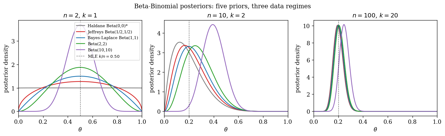
The picture is the classical one: at $n = 2$ the five posteriors are visibly different; by $n = 100$ four of them are virtually indistinguishable and only the strong $\mathrm{Beta}(10, 10)$ retains noticeable pull on the posterior mode. The MLE $k/n$ (dashed vertical) is the same in each regime, and the posteriors converge to it.

The catch with Haldane is failure at $k = 0$, which we illustrate separately:

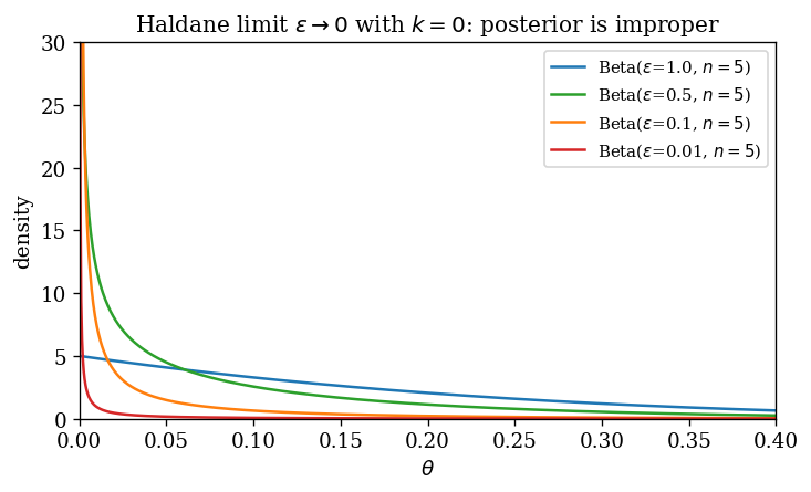
As $\epsilon \to 0$ in $\mathrm{Beta}(\epsilon, n)$, the would-be posterior mass concentrates at $\theta = 0$ and refuses to normalise: there is no probability density that the limit can be. This is the propriety theorem of §4 in action.

E2 — Bernardo missing information

We numerically verify the theorem of §6.5 / §8.2. For each candidate prior $\pi$, we draw $\theta \sim \pi$, then $k \sim \mathrm{Binomial}(n, \theta)$, and compute $\mathrm{KL}(p(\theta\mid k) \,\Vert\, \pi(\theta))$ in closed form for the Beta family. Averaging over $8000$ Monte Carlo draws gives an estimate of the missing-information functional $I_n(\pi)$.

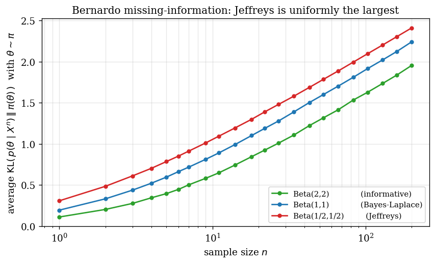
The three curves all grow like $\tfrac12 \log n$ (consistent with the $(d/2)\log n$ leading term of equation (20) for $d = 1$), but they differ in a constant. The constant is largest for Jeffreys, smaller for the uniform Bayes–Laplace, and smallest for the informative $\mathrm{Beta}(2, 2)$, matching the analytic formula

$$ I_n(\pi) \;\approx\; \tfrac12 \log n - \tfrac12 \log(2\pi e) - \tfrac12\bigl[\psi(\alpha) + \psi(\beta) - 2\psi(\alpha+\beta)\bigr] + h(\pi) + o(1), \tag{34} $$

with the variational maximum at $\pi \propto \sqrt{I(\theta)}$. The empirical ordering Jeffreys $>$ Uniform $>$ $\mathrm{Beta}(2,2)$ persists at every $n$ shown, with a constant offset of about $0.15$ between Jeffreys and Uniform — exactly what (34) predicts.

E3 — Frequentist coverage of Normal credible intervals

For $\mathcal N(\mu, \sigma^2)$ with both parameters unknown, the two competing noninformative priors are Jeffreys’ joint $\pi_J \propto 1/\sigma^2$ and Bernardo’s reference $\pi_R \propto 1/\sigma$. The marginal posteriors of $\mu$ under data $x_1, \ldots, x_n$ from $\mathcal N(0, 1)$ are (from §8.3)

• Reference: $\mu \mid x \sim t_{n-1}(\bar x, s^2_{\mathrm{unb}}/n)$ — identical to the frequentist $t$-interval.
• Jeffreys joint: $\mu \mid x \sim t_n(\bar x, s^2_{\mathrm{MLE}}/n)$ — wrong degrees of freedom and wrong scale.

We draw $8000$ datasets at each $n \in \{3, 5, 10, 30, 100\}$ and report the empirical coverage of the $95\%$ credible interval for $\mu$ under each prior:

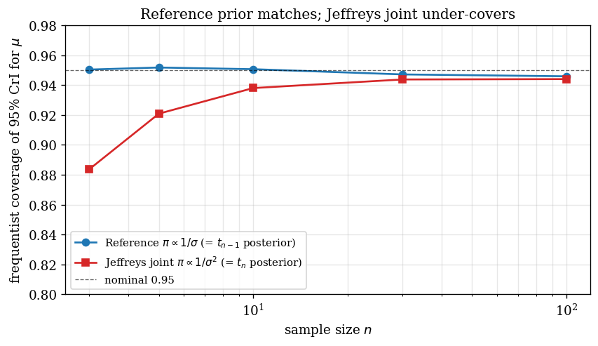
The reference-prior coverage is at the nominal $0.95$ at every $n$ (it has to be: the credible interval is the frequentist interval). The Jeffreys-joint coverage is $0.88$ at $n = 3$, climbing to $0.94$ at $n = 100$. The under-coverage is not a numerical artefact; it is the exact consequence of having one extra degree of freedom and an MLE-scale instead of unbiased-scale in the $t$ distribution.

The CrI-width distribution at $n = 5$ shows how the two priors differ quantitatively:

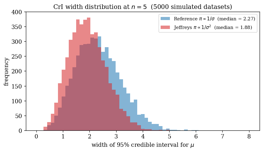
Jeffreys-joint produces narrower (and wrong) intervals; reference produces wider (and correctly calibrated) intervals.

E4 — The arc-length picture

The Bernoulli statistical manifold has finite Fisher arclength $\pi$ (equation (27)), and the natural arclength coordinate is $\phi = 2\arcsin\sqrt\theta$.

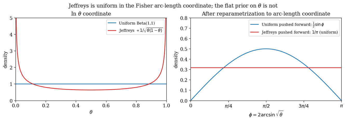
Left panel, $\theta$-coordinate: the Jeffreys density (red) has the U-shape $1/[\pi\sqrt{\theta(1-\theta)}]$, with infinite spikes at the boundaries. The flat $\mathrm{Beta}(1,1)$ density (blue) is constant.

Right panel, $\phi$-coordinate (arclength): the Jeffreys density pushes forward to the uniform $1/\pi$ on $[0, \pi]$, while the flat $\theta$-prior pushes forward to $\tfrac12 \sin\phi$ — not uniform. So in the parametrisation-free coordinate, the Jeffreys prior is the unique uniform measure and the Bayes–Laplace flat prior is warped.

We can visualise the Fisher metric directly:

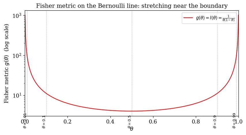
The metric $g(\theta) = 1/[\theta(1-\theta)]$ blows up at the boundaries, which is what stretches the manifold and forces the Jeffreys prior to put more mass at the endpoints when expressed in $\theta$-coordinates. In arclength coordinates the stretching has been absorbed into the change of variable and the prior is flat.

E5 — Shrinkage and the sufficient-statistic interpretation

To close the loop with the conjugate prior interpretation of §3, we show the posterior mean of $\theta$ as a function of $n$ for fixed true $\theta = 0.3$, under five Beta priors:

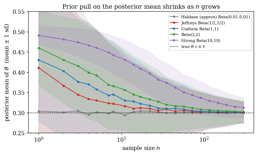
For each $n$ and each prior, we simulate $2000$ datasets, compute the posterior mean by (7), and plot the mean $\pm 1\,\mathrm{sd}$. The strong prior $\mathrm{Beta}(10, 10)$ has prior mean $0.5$ and is pulled towards the true $0.3$ only slowly — its posterior mean is still around $0.4$ at $n = 30$. The weak priors converge to $0.3$ from below (Haldane, Jeffreys) or are unbiased throughout (Bayes–Laplace). The convergence rate is exactly $(\alpha + \beta)/(\alpha + \beta + n)$, the prior weight in (7).

A worked example: dice throws

The chapters above are theory-heavy. To make sure the machinery is loaded into intuition rather than just notation, we walk through a single Bayesian problem end-to-end — a deliberately small one, where every number can be checked by hand, and where the coordinate-dependence pitfall of “flat” priors shows up as a concrete numerical disagreement.

The question

You are handed a six-sided die that may or may not be fair. You throw it ten times and observe a $6$ on two of those throws. What is $\theta := P(X = 6)$?

The model is $X_i \sim \mathrm{Bernoulli}(\theta)$ for $i = 1, \ldots, n = 10$, with $k = \sum X_i = 2$. The frequentist answer is the MLE $\hat\theta = k/n = 0.20$. A perfectly fair die would have $\theta = 1/6 \approx 0.167$. Bayesian estimation gives us a principled language to combine the data and our prior belief about how fair the die might be.

Four priors, four posteriors

We try four Beta priors. Two are textbook noninformative candidates (Bayes–Laplace flat and Jeffreys), one is the improper limit (Haldane), and one is a strongly informative prior expressing “I believe this die is fair.” By the conjugacy formula of §3 (equation (7)), each posterior is $\mathrm{Beta}(\alpha + k, \beta + n - k)$ and the posterior mean is the convex combination of prior mean and MLE with weight $(\alpha+\beta)/(\alpha+\beta+n)$ on the prior.

Prior $\pi(\theta)$	Pseudo-sample size $\alpha+\beta$	Posterior	Posterior mean
$\mathrm{Beta}(1, 1)$ — Bayes–Laplace flat	$2$	$\mathrm{Beta}(3, 9)$	$0.250$
$\mathrm{Beta}(0, 0)$ — Haldane (improper)	$0$	$\mathrm{Beta}(2, 8)$	$0.200$ (= MLE)
$\mathrm{Beta}(1/2, 1/2)$ — Jeffreys	$1$	$\mathrm{Beta}(2.5, 8.5)$	$\approx 0.227$
$\mathrm{Beta}(10, 50)$ — “fair die belief”	$60$	$\mathrm{Beta}(12, 58)$	$\approx 0.171$

The pattern is the one the chapter on conjugate priors promised: the hyperparameters $(\alpha, \beta)$ act exactly like pseudo-counts of past observations. The strong “fair die” prior is equivalent to having secretly thrown the die 60 times and seen 10 sixes — the new 10 throws are absorbed into that pseudo-history but barely move the posterior mean. The Bayes–Laplace flat prior is equivalent to having seen 2 throws — easily overwhelmed by real data. Jeffreys sits between them, with just enough weight to soften the MLE without overriding it.

The puzzle of “flat”

Now the part that the chapter on the noninformative landscape (§5) signposted as a trap. The Bayes–Laplace and Haldane priors are both informally described as “uninformative” — and they disagree about the posterior mean by $0.25$ vs $0.20$, a $25\%$ difference on the same data. Why?

Consider three coordinates on the same Bernoulli parameter:

• $\theta \in (0, 1)$ — the probability itself.
• $\eta = \log\!\dfrac{\theta}{1 - \theta} \in (-\infty, \infty)$ — the log-odds. A modeller working with logistic regression would consider $\eta$ the more natural coordinate.
• $\phi = 2\arcsin\sqrt{\theta} \in (0, \pi)$ — the Fisher arc-length coordinate from §7.

A prior is a measure on the parameter space, not a function of the coordinate, so changing coordinates changes the density by the Jacobian. With $d\theta / d\eta = \theta(1-\theta)$, a prior that is flat in $\theta$ becomes

$$ \pi(\eta) \;=\; \pi(\theta(\eta))\cdot\left|\frac{d\theta}{d\eta}\right| \;=\; 1 \cdot \theta(1-\theta) \;=\; \frac{e^{-\eta}}{(1 + e^{-\eta})^2}, \tag{35} $$

i.e. a logistic bell peaked at $\eta = 0$, which is $\theta = 0.5$. The $\eta$-modeller would look at this and say “you are putting a strong prior on the die being fair.” A prior that is flat in $\eta$, conversely, pushes forward to

$$ \pi(\theta) \;=\; 1 \cdot \left|\frac{d\eta}{d\theta}\right| \;=\; \frac{1}{\theta(1-\theta)}, \tag{36} $$

which is exactly Haldane $\mathrm{Beta}(0, 0)$ — divergent at the boundaries, putting all its mass on “the die is almost-never a 6” or “the die is almost-always a 6”. The $\theta$-modeller would call this strongly informative in the opposite direction.

So two perfectly reasonable people, each invoking the principle of indifference in their preferred coordinate, get incompatible answers on this dice problem. This is the failure mode that Jeffreys exists to fix.

Why Jeffreys ducks the puzzle

Jeffreys’ rule says: compute the Fisher information and take its square root, in whatever coordinate you happen to be using. The reparametrisation-invariance theorem of §6.3 guarantees that the resulting prior does not depend on the coordinate. Let us verify this by hand on the dice example.

In the $\theta$-coordinate the Fisher information of Bernoulli is $I(\theta) = 1/[\theta(1-\theta)]$ (§6.4), so

$$ \pi_J(\theta) \;\propto\; \frac{1}{\sqrt{\theta(1-\theta)}} \;=\; \mathrm{Beta}\!\left(\tfrac12, \tfrac12\right). \tag{37} $$

In the $\eta$-coordinate the log-likelihood is $\log p(x \mid \eta) = x\eta - \log(1 + e^\eta)$, whose second derivative is $-\sigma(\eta)(1 - \sigma(\eta)) = -\theta(1-\theta)$. So $I(\eta) = \theta(1-\theta)$ and

$$ \pi_J(\eta) \;\propto\; \sqrt{\theta(1-\theta)}. \tag{38} $$

These look like different formulas. Are they the same prior measure? Push $(37)$ forward through the change of variables $\theta \mapsto \eta$, using $|d\theta/d\eta| = \theta(1-\theta)$:

$$ \pi_J(\eta) \;=\; \pi_J(\theta(\eta))\cdot \theta(1-\theta) \;=\; \frac{1}{\sqrt{\theta(1-\theta)}} \cdot \theta(1-\theta) \;=\; \sqrt{\theta(1-\theta)}, \tag{39} $$

which matches (38) exactly. Two different routes — “compute Jeffreys in $\theta$ then transform” and “compute Jeffreys directly in $\eta$” — produce the same physical prior. This is what the abstract theorem of §6.3 says, instantiated.

One picture of all three priors in all three coordinates

Prior specification	density in $\theta$	density in $\eta$	density in $\phi$
Flat in $\theta$ (Bayes–Laplace)	constant ✓	logistic bell	$\frac12 \sin\phi$
Flat in $\eta$ (Haldane improper)	$1 / [\theta(1-\theta)]$	constant ✓	$\cot(\phi/2)$, divergent
Jeffreys	$1/\sqrt{\theta(1-\theta)}$ (U-shape)	$\sqrt{\theta(1-\theta)}$ (bell)	constant ✓

Each row is a single prior; the three columns are three coordinate representations of it. The shaded cell in each row marks the coordinate in which the prior is flat — and only Jeffreys is flat in the coordinate that the model itself singles out, the arc-length $\phi$ in which the Fisher metric is Euclidean (§7). The Haldane row diverges at the boundaries of both $\theta$ and $\phi$, which is why its posterior is improper whenever the data lie at those boundaries (§4). Equivalently, only Jeffreys is the volume element of the statistical manifold, which is the geometric statement of equation (25).

Five things this example shows

1. The posterior calculation is mechanical in any conjugate setup. $\alpha \to \alpha + k$ and $\beta \to \beta + n - k$. The mathematics of the Bayesian update has no judgement in it.
2. Prior strength is just pseudo-sample size. $\alpha + \beta$ is “how many fictitious throws you imagined before seeing the data.” A strong prior is one that imagined many throws; a weak prior, few.
3. “Flat” is not coordinate-free. Bayes–Laplace and Haldane both claim indifference, but the dice problem makes their disagreement quantitative: posterior means of $0.25$ vs $0.20$ on the same data.
4. Jeffreys is the coordinate-free choice. It is the volume element of the Fisher metric. It assigns probability mass proportional to arc-length on the statistical manifold, which is the unique sense in which a uniform measure on the model is intrinsic.
5. For estimating all six face probabilities simultaneously, the same logic extends through Dirichlet conjugacy: $\mathrm{Dirichlet}(\alpha_1, \ldots, \alpha_K)$ + $\mathrm{Multinomial}(n_1, \ldots, n_K)$ data → $\mathrm{Dirichlet}(\alpha_1 + n_1, \ldots, \alpha_K + n_K)$. The Jeffreys prior on the simplex is $\mathrm{Dirichlet}(\tfrac12, \ldots, \tfrac12)$.

If after all of §2–§10 the recipe still felt abstract, this dice problem is the same recipe applied with $n = 10$, and every claim of the post becomes a number you can check.

Summary

Five takeaways, one per chapter.

Conjugacy is sufficient-statistic bookkeeping. The natural conjugate prior of an exponential family has hyperparameters $(\tau_0, \nu_0)$ that update by $\tau_0 \to \tau_0 + \sum T(x_i)$ and $\nu_0 \to \nu_0 + n$. Use it when you want a closed-form posterior and a clear shrinkage picture; do not use it merely because the posterior is tractable, since MCMC removes that constraint.

Improper priors need a propriety check. A posterior under an improper prior exists if and only if $m(x) < \infty$ for the observed $x$. This is data-dependent. Improper priors are fine for parameter estimation, never for Bayes factors or model selection.

Jeffreys is the volume element of the Fisher–Rao metric. It is coordinate-free by construction (the proof is the volume-form change-of-variables rule), and it is asymptotically the maximiser of the missing-information functional. In one dimension it equals the reference prior; in higher dimensions it may not.

Reference priors fix what Jeffreys gets wrong in higher dimensions by introducing an explicit ordering of parameters and constructing conditional Jeffreys priors sequentially. For Normal $(\mu, \sigma)$ this gives $1/\sigma$ instead of $1/\sigma^2$, which has the bonus property of matching the frequentist $t$-interval exactly. When in doubt, prefer the reference prior; it is rarely worse than Jeffreys and often strictly better.

“Objective Bayes” still requires judgement. There are at least five inequivalent uninformative-prior constructions (Jeffreys, reference, MaxEnt, probability-matching, formal rules), and Yang–Berger [ref 1] catalogues many more. The choice between them is a modelling decision, not a logical theorem, and pretending otherwise is the cleanest way to lose the trust of a sceptical reader.

References

1. Yang, R. and Berger, J. O. (1998). A Catalog of Noninformative Priors. ISDS Discussion Paper 97-42.
2. “Does the Bayesian posterior need to be a proper distribution?” — Cross Validated.
3. Cook, J. D. Compendium of Conjugate Priors.
4. “Difference between non-informative and improper priors” — Cross Validated.
5. Wasserman, L. Bayesian Inference (SML lecture notes).
6. “Choosing between uninformative beta priors” — Cross Validated.
7. Wilson, B. Noninformative Priors. NCSU Stat course notes.
8. Jordan, M. I. Bayesian Modeling and Inference (Lecture 7). UC Berkeley CS 260, Spring 2010.
9. “Why are Jeffreys priors considered noninformative?” — Cross Validated. (References Bernardo 1979 and Berger–Bernardo–Sun 2009.)
10. West, M. Priors and Posteriors. Duke STA 732 notes, Spring 2013.
11. Amari, S. (2016). Information Geometry and Its Applications. Applied Mathematical Sciences vol. 194, Springer.